Forrest M. Hoffman¹, Mariana Vertenstein², James B. White III¹, Patrick Worley¹, John Drake¹
¹Oak Ridge National Laboratory (ORNL)
²National Center for Atmospheric Research (NCAR)
January 13, 2004
The following are initial timing results for the vectorized version of
the Community
Land Model Version 2 (CLM2) (tag clm2_deva_51) run on
the Cray
X1 at Oak Ridge National
Laboratory's Center
for Computational Sciences (CCS). The purpose of these tests was
to gauge overall performance of the new CLM2 code and determine the
optimum configuration for runs at production resolutions (T42 and T85)
on the Cray X1 platform. The timing tests consist of a series of 90
day T42 and T85 offline runs of CLM2 varying both processor counts
(with and without OpenMP) and the clumps-per-process tuning parameter.
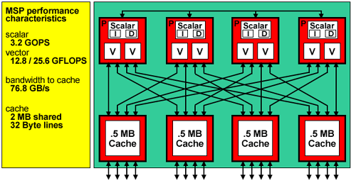
The processor used in the Cray X1 is called a multi-streaming processor or MSP. Each MSP consists of four tightly coupled scalar single-streaming processors (SSPs) and four external cache chips. Each SSP contains a dual-pipe vector unit (32-stage, 64-bits wide running at 800 MHz) and a 2-way superscalar unit running at 400 MHz. As a result, each MSP has a total of eight vector pipelines which can operate in parallel and deliver eight results per clock cycle. Code can be compiled to run directly on the SSPs (called SSP mode) or on the MSP (called MSP mode). When compiling for MSP mode, the Cray compilers automatically multi-stream concurrent loops where possible; however, users may also force streaming to occur for particular loops by inserting Cray Streaming Directives (CSDs) around those loops. All development and testing with CLM2 has been performed in MSP mode. In the discussion that follows, a "processor" on the Cray X1 refers to one MSP.
|
| Figure 1: The Cray X1 Multi-Streaming Processor (MSP) contains four single-streaming processors (SSPs) with 4×2 vector pipes. |
Each node in the Cray X1 contains four MSPs, 16-64 GB of globally-shared memory, and four I/O ports. A distributed set of routing switches controls all memory access within the node and access to the node interconnection network. Each node contains 32 network ports; each port supports 1.6 GBps peak bandwidth per direction.
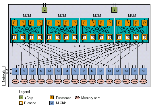 |
| Figure 2: The Cray X1 node consists of four MSPs and 16-64 GB of globally-shared memory. |
The Cray X1 system at ORNL, named Phoenix, has 64 SMP nodes for a total of 256 MSPs, 1024 GB of memory, and 3200 GFlop/s peak performance.
CLM2 may be built in a number of ways depending on the computer architecture and processor configuration to be used. Both MPI and OpenMP may be independently enabled or disabled. With both MPI and OpenMP disabled the model can run serially on a single processor. With MPI enabled and OpenMP disabled the model runs in distributed memory mode across a number of nodes. With MPI disabled and OpenMP enabled the model can run on a single shared memory symmetric multi-processor (SMP) node. With both MPI and OpenMP enabled, CLM2 runs in hybrid distributed/shared memory across a number of SMP nodes.
On the Cray X1, CLM2 can also be built with Cray Streaming Directives (CSDs). However, in CLM2 it happens that CSDs are used only around loops which also use OpenMP directives. As a result, OpenMP can be used only when CSDs are not. When compiling with OpenMP (ignoring CSDs), the compiler will still multi-stream concurrent loops within subroutines where possible. In CLM2 such loops tend to be in science subroutines contained in separate modules. Call to these science subroutines are typically contained within the higher-level loops in the driver module where OpenMP directives and CSDs are used. The performance impacts of CSDs versus OpenMP on the Cray X1 are described below.
In the performance tests that follow, six different configurations are used.
Note: The first two tests were not performed at T42 resolution, but all tests were performed at T85 resolution.
In all tests using multiple MSPs with OpenMP disabled, the number of MPI processes is equal to the number of MSPs used. With OpenMP enabled, the number of MPI processes and OpenMP threads is explicitly listed. Four threads were used for all tests with OpenMP enabled. The curves in the graphs below are all colored by the total number of MSPs used in the run. For instance, the curves for 32 MSPs (32 MPI processes and OpenMP disabled) and for 8 MPI processes with 4 OpenMP threads are both colored cyan.
The land model grid is decomposed into groups of gridcells
called clumps. These clumps are of approximately equal weight or
computational cost and are distributed among available MPI processes
providing a reasonably good load balance. The number of clumps defined
is proportional to the number of MPI processes and is established by the
clumps-per-process tuning parameter. When set to 1, a single clump is
defined for each process resulting in the maximum possible vector length.
Since the high-level loops in the driver module are over clumps, this
parameter allows for cache-friendly blocking. With OpenMP enabled,
this parameter should be set to the number of OpenMP threads (or to
something proportional to the number of threads) for best performance.
Similarly, with CSDs enabled on the Cray X1, clumps-per-process should
be set to 4. The clumps-per-process parameter may be set at run-time
using the namelist variable clump_pproc. If not set on the
namelist, clump_pproc will default to the maximum number
of OpenMP threads in future releases of CLM.
The clumps-per-process tuning parameter was varied between 1 and 32 for the performance tests below.
At T42 resolution, two sets of tests were performed: one set with CSDs enabled and one set with OpenMP enabled. In both cases, MPI was disabled for the 1 MSP test while MPI was utilized for the 2 through 32 MSP tests. The number of MSPs is equal to the number of MPI processes.
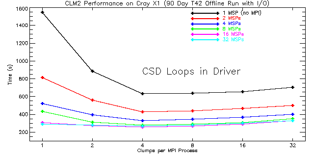 |
| Figure 3: Total run times for CLM2 using Cray Streaming Directives (CSDs) around high-level clump loops in the driver routine for 1 to 32 processors. The number of MPI processes is equal to the number of MSPs. The performance for fewer than four clumps per MPI process is expected to be poor since the SSPs are not fully utilized. |
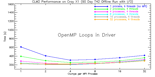 |
| Figure 4: Total run times for CLM2 using OpenMP directives around high-level loops in the driver routine for 1 to 32 MPI processes with four threads each. The number of Cray X1 nodes is equal to the number of processes shown here. The performance for fewer than four clumps per MPI process is expected to be poor since the four OpenMP threads are not fully utilized. |
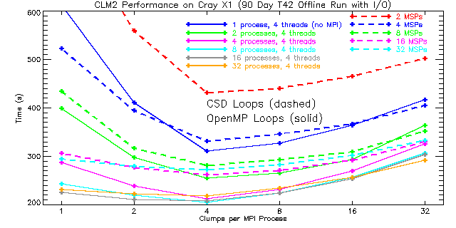 |
| Figure 5: A section of Figures 3 and 4 combined. Timings for CSD loops are shown as dashed curves while solid curves represent OpenMP timings. For the T42 problem size, performance turns over at 16 MSPs when using CSDs and at 32 MSPs when using OpenMP. The performance for fewer than four clumps per MPI process is expected to be poor. |
As expected, the best performance is obtained when using four clumps per MPI process irrespective of whether CSDs or OpenMP is used. For the CSD case this is due to the fact that each MSP has four SSPs while for the OpenMP timings four OpenMP threads per process were used. For the CSD case, performance degrades when moving from 16 to 32 MSPs. At that point the problem becomes too small, i.e., the vector length becomes too short for continued scaling, and MPI communications becomes a bottleneck. On the other hand, the OpenMP scaling is better. Peak performance for OpenMP is obtained with 8 processes and 4 threads (8 SMP nodes containing 4 MSPs each for a total of 32 MSPs). Moreover, OpenMP performance is always better than that obtained using CSDs around the high-level clump loops in CLM2. This result is somewhat surprising because the overhead associated with OpenMP is higher than that associated with CSDs. However, the better performance and improved scaling with OpenMP is probably due to the fact that the compiler does a good job of multi-streaming lower-level loops throughout the scientific subroutines and because the amount of MPI communication is reduced. By making fairly good use of the SSPs in lower-level loops, OpenMP provides an alternative mechanism for parallelizing the high-level clump loops resulting in improved performance overall.
Since the IPCC and other studies will be using T85 resolution, the same timing tests were performance again at T85. In order to gauge the value of CSDs used in conjunction with clumping, the model was also run with CSDs and OpenMP disabled. In this configuration, multi-streaming of lower-level science subroutine loops is still performed; however, the high-level clump loops in the driver module are not executed concurrently. As before, a set of tests using CSDs and OpenMP were run varying processor count and the clumps-per-process tuning parameter.
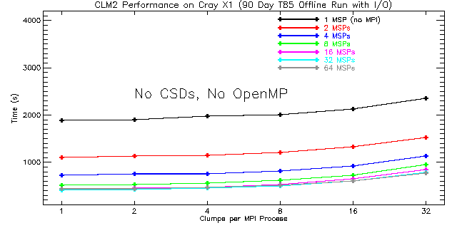 |
| Figure 6: Total run times for CLM2 with CSDs and OpenMP both disabled for 1 to 64 MSPs. The number of MPI processes is equal to the number of MSPs used. This problem scales to 32 MSPs with 1 clump per process yielding the best performance. |
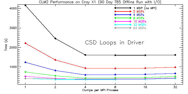 |
| Figure 7: Total run times for CLM2 using Cray Streaming Directives (CSDs) around high-level loops in the driver routine for 1 to 64 processors. The number of MPI processes is equal to the number of MSPs used. The performance for fewer than four clumps per MPI process is expected to be poor since the SSPs are not fully utilized. |
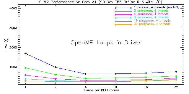 |
| Figure 8: Total run times for CLM2 using OpenMP directives around high-level loops in the driver routine for 1 to 32 MPI processes with four threads each. The number of Cray X1 nodes is equal to the number of processes shown here. The performance for fewer than four clumps per MPI process is expected to be poor since the four OpenMP threads are not fully utilized. |
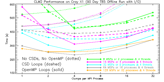 |
| Figure 9: A section of Figures 6, 7, and 8 combined. The dotted curves represent runs with CSDs and OpenMP disabled, the dashed curves represent runs using CSDs, and the solid curves represent runs using OpenMP. For the T85 problem size, performance turns over at 32 MSPs when using CSDs and at 64 MSPs when using OpenMP. The performance for fewer than four clumps per MPI process is expected to be poor for the CSD and OpenMP cases. |
As before, the best performance is obtained when using four clumps per process irrespective of whether CSDs or OpenMP is used. However, when CSDs and OpenMP are both disabled, the best performance is obtained with one clump per MPI process. This makes the vectors as long as possible given the decomposition across MPI processes. Nevertheless, on the Cray X1 an average of 15.6% better performance is realized (with similar scaling) by using clumping and enabling CSDs around high-level clump loops to explicitly utilize the four SSPs on each MSP. This result demonstrates the value of using CSDs when OpenMP is not used.
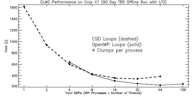 |
| Figure 10: Timings for 90 day T85 runs by processor (MSP) count. The dashed curve represents runs using CSDs, and the solid curve represents runs using OpenMP. For all these runs, 4 clumps per process were used. As a result, the performance for fewer than four MSPs is expected to be poor. |
As can be seen from Figure 10, good scaling for the T85 problem size is obtained up to 32 MSPs for the CSD case and to 64 MSPs for the OpenMP case. This is twice the processor count of the turnover seen at T42 resolution. As in the T42 tests, OpenMP performance and scaling at T85 are better than that obtained using CSDs for the same high-level clump loops in the driver module. MPI performance on the Cray X1 limits scaling beyond 32 MSPs, but adding shared-memory processors via OpenMP improves scaling to 64 MSPs (i.e., 16 MPI processes and 4 OpenMP threads). Despite the additional overhead associated with OpenMP, it appears that the compiler does a good job of multi-streaming lower-level loops in science subroutines (thereby keeping the SSPs sufficiently busy) so that using OpenMP to parallelize high-level clump loops results in better performance overall.
Table 1 contains a complete profile report of CLM2 running on a single
MSP with Cray Streaming Directives (CSDs) enabled. This report provides
a good overview of the routines that consume the largest amount of real
run time. The most costly routine is gettimeofday which is
used by the timing utilities. It is known that gettimeofday
is particularly expensive on the Cray X1. Running with timers based on
rtc calls or with timers disabled could noticeably improve
model performance. The second routine, %__rtor_vv, appears
to be a real-to-real vector memory copy routine. The third routine,
canopyfluxes, is the most expensive scientific subroutine.
This routine is known to represent the majority of the calculations in
the present version of CLM, and it has been extensively optimized.
   Samp% | Cum.Samp% |  Samp |SSP=0
                             |Function
                             |Caller
|--------------------------------------
| 100.0% |    100.0% | 59330 |Total
|--------------------------------------
|  10.7% |     10.7% |  6368 |gettimeofday
|  10.0% |     20.8% |  5944 |%__rtor_vv
|   7.1% |     27.9% |  4233 |canopyfluxes@canopyfluxesmod_
|   6.7% |     34.6% |  3966 |updateinput@rtmmod_
|   5.6% |     40.1% |  3293 |%__alog
|   5.3% |     45.4% |  3135 |areaovr_point@areamod_
|   5.0% |     50.4% |  2966 |pft2col@pft2colmod_
|   4.6% |     55.0% |  2725 |rtmriverflux@rtmmod_
|   4.3% |     59.3% |  2540 |mkmxovr@areamod_
|   2.7% |     62.0% |  1585 |soiltemperature@soiltemperaturemod_
|   2.6% |     64.6% |  1543 |areaave@areamod_
|   2.4% |     67.0% |  1433 |phasechange@soiltemperaturemod_
|   2.3% |     69.3% |  1368 |%__exp
|   1.9% |     71.2% |  1117 |biogeophysics2@biogeophysics2mod_
|   1.9% |     73.0% |  1115 |stomata@canopyfluxesmod_
|   1.8% |     74.9% |  1084 |frictionvelocity@frictionvelocitymod_
|   1.7% |     76.6% |  1019 |soilwater@soilhydrologymod_
|   1.7% |     78.2% |   990 |tridiagonal@tridiagonalmod_
|   1.6% |     79.9% |   970 |update_hbuf_field@histfilemod_
|   1.5% |     81.3% |   866 |soilthermprop@soiltemperaturemod_
|   1.4% |     82.7% |   822 |combinesnowlayers@snowhydrologymod_
|   1.2% |     83.9% |   723 |lseek
|   1.2% |     85.1% |   705 |__read
|   1.1% |     86.3% |   672 |__write
|   1.0% |     87.3% |   600 |update_hbuf@histfilemod_
|   0.6% |     87.9% |   383 |surfacerunoff@soilhydrologymod_
|   0.6% |     88.6% |   372 |vec2xy@mapxy_
|   0.6% |     89.2% |   357 |%__atan
|   0.5% |     89.7% |   307 |driver_
|   0.5% |     90.2% |   293 |__atan
|   0.5% |     90.6% |   283 |areaovr@areamod_
|   0.5% |     91.1% |   276 |hydrology2@hydrology2mod_
|   0.5% |     91.6% |   269 |drainage@soilhydrologymod_
|   0.4% |     92.0% |   251 |atm_readdata@atmdrvmod_
|   0.4% |     92.4% |   248 |snowwater@snowhydrologymod_
|   0.4% |     92.8% |   224 |dividesnowlayers@snowhydrologymod_
|   0.4% |     93.2% |   222 |makel2a@lnd2atmmod_
|   0.4% |     93.5% |   211 |__sin
|   0.3% |     93.8% |   200 |%__alog10
|   0.3% |     94.2% |   195 |biogeophysics1@biogeophysics1mod_
|   0.3% |     94.5% |   190 |baregroundfluxes@baregroundfluxesmod_
|   0.3% |     94.7% |   149 |_ld_read
|   0.2% |     95.0% |   131 |initdecomp@decompmod_
|   0.2% |     95.2% |   130 |_stride_dv
|  Truncated because cumulative % of Samp exceeds 95.
|======================================
|
The updateinput, areaovr_point,
mkmxovr, areaave routines provide data
exchange and interpolation functionality for the River Transport Model
(RTM) while rtmriverflux runs the RTM. The data exchange
and interpolation functions, which have not been vectorized, are used
repeatedly when running CLM2 in offline mode; however, they are called
only during initialization when run in the fully coupled CCSM mode. The
pft2col routine accumulates data from the plant functional
type (PFT) sub-grid level to the column level.
Table 2 shows the top 10 routines for the same 90 day run using 2
MSPs with CSDs enabled. MPI is used for communication, and already
MPI_Gatherv and MPI_Bcast are showing up as
the 7th and 8th position in the report. A small portion of this time
is attributable to synchronization, but it is clear that MPI performance
could be improved. CLM2 has very good load balancing so synchronization
takes very little time. MPI_Gatherv is used each time
step to generate a temperature diagnostic, and it is used to accumulate
data for history output. MPI_Bcast is used to distribute
atmospheric forcing data read from disk by the master process to all
processes on a monthly basis.
   Samp% | Cum.Samp% |  Samp |SSP=0
                             |Function
                             |Caller
|--------------------------------------
| 100.0% |    100.0% | 82521 |Total
|--------------------------------------
|  13.8% |     13.8% | 11372 |gettimeofday
|   7.8% |     21.6% |  6459 |areaovr_point@areamod_
|   7.1% |     28.7% |  5822 |%__rtor_vv
|   6.4% |     35.1% |  5278 |mkmxovr@areamod_
|   5.3% |     40.4% |  4393 |updateinput@rtmmod_
|   5.3% |     45.7% |  4379 |canopyfluxes@canopyfluxesmod_
|   5.3% |     50.9% |  4334 |MPI_CRAY_gatherv
|   4.9% |     55.8% |  4023 |MPI_CRAY_bcast
|   3.9% |     59.7% |  3181 |rtmriverflux@rtmmod_
|   3.8% |     63.5% |  3176 |pft2col@pft2colmod_
     .           .        .        .
     .           .        .        .
     .           .        .        .
|
As can be seen from Table 3, MPI_Bcast and
MPI_Gatherv are second and third most expensive routines
when run on 32 MSPs. Only gettimeofday represents more time
samples. MPI_Allgatherv, used after each run of RTM, appears
at number 10. With 32 MPI processes, MPI routines and interpolation for
RTM dominate run time. While some additional time may be attributable
to a slightly larger load imbalance than when using 2 processes, at 32
MPI processes communication time appears to exceed calculation time.
   Samp% | Cum.Samp% |   Samp |SSP=0
                              |Function
                              |Caller
|---------------------------------------
| 100.0% |    100.0% | 829295 |Total
|---------------------------------------
|  21.9% |     21.9% | 181986 |gettimeofday
|  15.2% |     37.1% | 125741 |MPI_CRAY_bcast
|  13.5% |     50.6% | 112289 |MPI_CRAY_gatherv
|  12.3% |     63.0% | 102158 |areaovr_point@areamod_
|  10.5% |     73.4% |  86886 |mkmxovr@areamod_
|   7.3% |     80.8% |  60740 |rtmriverflux@rtmmod_
|   4.0% |     84.8% |  33180 |areaave@areamod_
|   2.3% |     87.0% |  18867 |atm_readdata@atmdrvmod_
|   1.1% |     88.2% |   9518 |areaovr@areamod_
|   1.1% |     89.3% |   9149 |MPI_Allgatherv
     .           .        .        .
     .           .        .        .
     .           .        .        .
|